How EM (Expectation Maximization) Method Works for Clustering

Background

To get strong understanding about EM concept, digging from the mathematical derivation is good way for it. But before it, let’s put the condition first. EM method is intended for clustering, and the most familiar method is k-means clustering, which is the special case of EM method that use Gaussian mixture to model the cluster areas and using hard clustering instead of soft clustering.

See picture below.

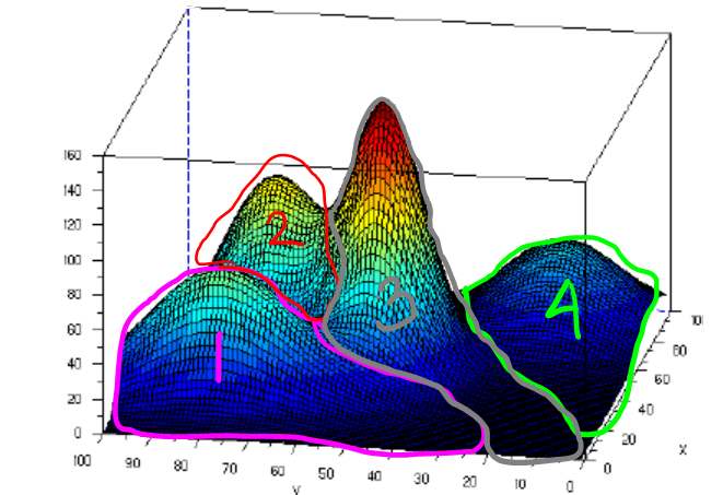
Picture above shows that we have 4 clusters where each cluster is modeled using Gaussian. To determine the data belongs to which cluster, we can just determine by finding the maximal value among the fourth Gaussian value. The data will be clustered to the cluster whose Gaussian value is maximal in that location. For instance, the area in the pink line boundary has maximal Gaussian value which is from Gaussian value in cluster 1, likewise for other clusters. Doing this type of clustering, the clustering boundary may intersects each others and taking cluster whose the value is maximal, is called soft clustering. Whereas for hard clustering, the boundary doesn’t intersect each others. To be able to cluster like that, we need parameters mean and variance of all those 4 Gaussian distributions, given data set input without class label. And we can achieve this by using EM method.

Ok, we already get the basic idea how it works. Next, we will dig through the mathematical approach. To do this, we choose a case which its distribution is Bernoulli distribution so that it will be much easier to derive. If in Gaussian we need parameter mean and variance, in Bernoulli distribution, we need parameter $P$ and $\lambda$ . To get those parameter, we can achieve by doing MLE. We can start by doing MLE both in labelled data training and unlabeled data training. Let’s do MLE in labelled data first. Here is the setup.

$x=\begin{Bmatrix} 1,0,1,1,0,0,1,0,1,0\end{Bmatrix}\\\\z=\begin{Bmatrix} 0,1,0,1,0,0,1,0,1,1\end{Bmatrix}$

Given two tossing coins $c_0, c_1$ result $=x$ , $z$ tells us from what coin it is. If $z=0$ , it’s from $c_0$ , and if $z=1$ , it’s from $c_1$ . And we need one more parameter which is the probability of $c_0$ is used. Let’s denote it with $\lambda$ . As a consequence, probability that $c_1$ is used is $(1-\lambda)$ .

After we get all setups, we will try to do MLE (Maximum Likelihood Estimation). We can construct our likelihood as Bernoulli probability as follows.

$likelihood =P(x|P_{c_0},P_{c_1},\lambda, z)\\\\likelihood =\prod_{i=1}^{n}(\lambda P_{c_0}^{x_i}(1-P_{c_0})^{1-x_i})^{1-z_i}\,((1-\lambda)P_{c_1}^{x_i}(1-P_{c_1})^{1-x_i})^{z_i}$

Likelihood formula above is really straightforward. If you find it difficult to understand, you may check Bernoulli distribution we already talk here. Next, we will do MLE by maximizing the likelihood to find parameter $\lambda, P_{c_0},$ and $P_{c_1}$ that maximize our likelihood. To do that, as we already did many times before, we will bring the likelihood equation to log form. Here we go.

$likelihood=\sum_{i=1}^{n}[(1-z_i)ln(\lambda P_{c_0}^{x_i}(1-P_{c_0}^{x_i})^{1-x_i})+z_iln(1-\lambda)P_{c_1}^{x_i}(1-P_{c_1})^{1-x_i}]\\\\ likelihood=\sum_{i=1}^{n}[(1-z_i)ln\lambda +(1-z_i)x_ilnP_{c_0}+(1-z_i)(1-x_i)ln(1-P_{c_0})\\ \hspace*{60pt} +z_iln(1-\lambda) +z_ix_ilnP_{c_1}+z_i(1-x_i)ln(1-P_{c_1})]$

To find $\lambda, P_{c_0},$ and $P_{c_1}$ that maximize our likelihood, we can take first differential w.r.t $\lambda, P_{c_0},$ and $P_{c_1}$ respectively, and make it equal to zero. Let’s do for $\lambda$ first. Here we go.

$\frac{\delta [likelihood]}{\delta \lambda}=\frac{\delta[\sum_{i=1}^{n}(1-z_i)ln \lambda + z_i ln(1-\lambda)]}{\delta \lambda}=0$

We get formula above because the other terms don’t have $\lambda$ , so they will just become zero it we take first differential w.r.t $\lambda$ . And let’s proceed our derivation to get $\lambda$ .

$\frac{\delta [likelihood]}{\delta \lambda}=\frac{\delta [ln \lambda\sum_{i=1}^{n}(1-z_i) + ln(1-\lambda) \sum_{i=1}^{n} z_i]}{\delta \lambda}=0\\\\ \frac{1}{\lambda}\sum_{i=1}^{n}(1-z_i)=\frac{1}{(1-\lambda)}\sum_{i=1}^{n}z_i\\\\ (1-\lambda)\sum_{i=1}^{n}(1-z_i)=\lambda \sum_{i=1}^{n} z_i\\\\ \sum_{i=1}^{n}(1-z_i)-\lambda\sum_{i=1}^{n}(1-z_i)=\lambda \sum_{i=1}^{n} z_i\\\\ \sum_{i=1}^{n}(1-z_i)-\lambda\sum_{i=1}^{n}(1-z_i)=\lambda \sum_{i=1}^{n} z_i+\lambda\sum_{i=1}^{n}(1-z_i)\\\\ \sum_{i=1}^{n}(1-z_i)=\lambda \sum_{i=1}^{n} [z_i+(1-z_i)]\\\\ \sum_{i=1}^{n}(1-z_i)=\lambda \sum_{i=1}^{n}1\\\\ \sum_{i=1}^{n}(1-z_i)=\lambda n\\\\ \boxed{\lambda=\frac{\sum_{i=1}^{n}(1-z_i)}{n}}$

As for other parameters $P_{c_0}$ and $P_{c_0}$ , we can just do the similar by differentiating the likelihood w.r.t $P_{c_0}$ and $P_{c_0}$ respectively and make it equal to zero. By doing that, we will get the final result as follows.

$\boxed {P_{c_0}=\frac{\sum_{i=1}^{n}x_i-\sum_{i=1}^{n}z_ix_i}{n-\sum_{i=1}^{n}z_i}}$ , and $\boxed {P_{c_0}=\frac{\sum_{i=1}^{n}z_ix_i}{\sum_{i=1}^{n}z_i}}$ .

Unlabeled data (no data z) → using EM method

What we did in the “background” discussion above is when we have class data label, which is denoted by $z$ . What if we don’t have it? We use EM method. Here is the setup.

$P(z_i=c_0, x|\lambda,P_{c_0})=\lambda P_{c_0}^{x_i}(1-P_{c_0})^{(1-x_i)}\\\\ P(z_i=c_1,x|\lambda,P_{c_1})=(1-\lambda) P_{c_1}^{x_i}(1-P_{c_1})^{(1-x_i)}\\\\ w_{{c0}_i}=\frac{P(z_i=c_0,x|\lambda,P_{c_0})}{P(z_i=c_0,x|\lambda,P_{c_0})+P(z_i=c_1,x|\lambda,P_{c_1})}\\\\ w_{{c1}_i}=\frac{P(z_i=c_1,x|\lambda,P_{c_1})}{P(z_i=c_0,x|\lambda,P_{c_0})+P(z_i=c_1,x|\lambda,P_{c_1})}$

The first and second line formula are the joint probability of cluster 0 and cluster 1 respectively. Because we don’t have data label $z$ , we will use weighting value, that is also often called responsibility. We will MLE again for this case, unlabeled data. Our likelihood will be:

$likelihood = \sum_{i=1}^{n} [w_{{c0}_i} ln \lambda P_{c_0}^{x_i}(1-P_{c_0})^{1-x_i}+(1-w_{{c0}_i})ln (1-\lambda) P_{c_1}^{x_i}(1-P_{c_1})^{1-x_i}]$

Doing MLE that is similar what we did before in labelled data case, we will get the final result as follows.

$\boxed{\lambda=\frac{\sum_{i=1}^{n}w_{{c0}_i}}{n}}, \boxed{P_{c_0}=\frac{\sum_{i=1}^{n}w_{{c0}_i}x_i}{\sum_{i=1}^{n}w_{{c0}_i}}}, \boxed{P_{c_1}=\frac{\sum_{i=1}^{n}x_i-\sum_{i=1}^{n}w_{{c0}_i}x_i}{n-\sum_{i=1}^{n}w_{{c0}_i}}}$

And finally, our two clusters can be constructed by using parameters $P_{c_0}$ and $P_{c_0}$ above using Bernoulli distribution to model our cluster. But, how to get them? To get them we need weighting value $w_{{c0}_i}$ , but, to get $w_{{c0}_i}$ need $\lambda$ , $P_{c_0}$ and $P_{c_0}$ . It’s like chicken-egg problem then, looping! To solve this, we can use EM algorithm as follows.

Initiate our model parameters. In this case, we use Bernoulli to model our cluster areas, thus those parameters are mixing coefficient $\lambda$ , $P_{c_0}$ , and $P_{c_1}$ . In case we use Gaussian to model our cluster, those parameters should be mean and variance of each Gaussians, aslo the mixing coefficient.
After that, we can calculate weighting value (responsibility), in our case would be $w_{{c0}_i}$ .
After we get weighting value $w_{{c0}_i}$ , we can calculate new parameters $\lambda$ , $P_{c_0}$ , and $P_{c_1}$ (again, if we use Gaussian to model cluster areas, those new parameters would be mean, variance of each Gaussians and the mixing coefficient).
And then this process keep repeated iteratively by doing step (2) and (3) until it converged. We will get the final parameter values of our cluster area models. In our case will be parameters $\lambda, P_{c_0}$ and $P_{c_0}$ that can be used by us to construct our two cluster areas. Each data belongs to cluster whose joint probability value is the highest one. Voila!

Relation between EM method and k-means clustering

From discussion above, we already know that EM is constructed using mixture of distribution model, such as BMM (Bernoulli Mixture Model) and GMM (Gaussian Mixture Model). Like we already mention above, k-means clustering is just special case of EM method, which is using GMM and hard clustering. Instead of calculating and giving weight/responsibility value to each data for each clusters, we will set weight/responsibility value to 1 for data input belonging to cluster whose mean value is the nearest to that data input, and set zero weight value for other clusters. And the are just same. Here are the steps summary for doing k-Means clustering.

Specify how many clusters, and initiate means for each clusters. Each cluster will have means that is same number with the given data input dimension.
Assign each data input into each cluster. Each data input belongs to cluster whose the mean is the nearest one.
After we do step (2), we will members in each clusters. Then, re-calculate the means of each there clusters.
Iterate step (2) and (3) until it converged. Converged in k-means is when the means of each clusters don’t change again in the next iteration compared to the previous one.

In k-means, the are some considerations:

We need to specify how many clusters we want to make, and we need to specify means of each clusters.
Different means initialization may give different final result clusters
It is possible that we will have zero member in certain cluster
k-means lacks robustness to outliers. Because k-means will treat with same weight for normal data and outliers data. Whereas, for EM method, it will treat with different weight, so, it is more robust to outliers.

How EM (Expectation Maximization) Method Works for Clustering

Background

Unlabeled data (no data z) → using EM method

Relation between EM method and k-means clustering

Published by ardianumam

Leave a comment Cancel reply

Background

Unlabeled data (no data z) → using EM method

Relation between EM method and k-means clustering

Share this:

Related

Published by ardianumam

Leave a comment Cancel reply