Apache Spark Tutorial for Big Data Analytics

Hi!

This post will provide you video series talking about how we can do big data analytics using Apache Spark.

Machine Learning from The Scratch using Python

This post provides video series how we can implement machine learning algorithm from the scratch using python. Up to know, the video series consist of clustering methods, and will be continued for regression, classification and pre-processing methods, such as PCA. Check this out!

*this is in playlist mode. So, you can check other videos in the playlist navigation.

Continue reading →

Estimator for Mean and Variance of Sampled Data

Estimator is a statistic, usually in a function of the data, that is used to infer the value of an unknown parameter in a statistical model. During this post, we will talk about estimator for mean and variance of sampled data. We can determine a good estimator by calculating the bias of it. A good estimator should give bias closed to zero. Let $\theta$ is parameter we want to estimate/observe, our estimator result will be $\hat{\theta}$ . The bias of our estimator is defined as follows.

$bias = E[\hat{\theta}]-\theta$

We will use bias formula above to check whether our estimator is good or not. And during this post, we will check our estimator we already derived by MLE here, which are mean and variance. Let’s write them first.

$\mu_{MLE}=\hat{\mu}=\frac{1}{n}\sum_{i=1}^{n}x_i\\\\ \sigma^2_{MLE}=\hat{\sigma}^2=\frac{1}{n}\sum_{i=1}^{n}(x_i-\hat{x})^2$

where $\bar{x}=\mu$ and $\hat{x}=\hat{\mu}$ Continue reading “Estimator for Mean and Variance of Sampled Data” →

How EM (Expectation Maximization) Method Works for Clustering

Background

To get strong understanding about EM concept, digging from the mathematical derivation is good way for it. But before it, let’s put the condition first. EM method is intended for clustering, and the most familiar method is k-means clustering, which is the special case of EM method that use Gaussian mixture to model the cluster areas and using hard clustering instead of soft clustering.

See picture below.

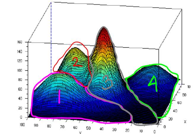
Picture above shows that we have 4 clusters where each cluster is modeled using Gaussian. To determine the data belongs to which cluster, we can just determine by finding the maximal value among the fourth Gaussian value. The data will be clustered to the cluster whose Gaussian value is maximal in that location. For instance, the area in the pink line boundary has maximal Gaussian value which is from Gaussian value in cluster 1, likewise for other clusters. Doing this type of clustering, the clustering boundary may intersects each others and taking cluster whose the value is maximal, is called soft clustering. Whereas for hard clustering, the boundary doesn’t intersect each others. To be able to cluster like that, we need parameters mean and variance of all those 4 Gaussian distributions, given data set input without class label. And we can achieve this by using EM method. Continue reading “How EM (Expectation Maximization) Method Works for Clustering” →

How Logistic Regression Works for Classification (with Maximum Likelihood Estimation Derivation)

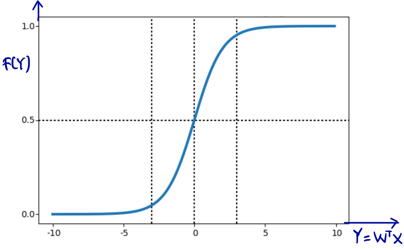
Logistic regression is an extension of regression method for classification. In the beginning of this machine learning series post, we already talked about regression using LSE here. To use regression approach for classification,we will feed the output regression $Y$ into so-called activation function, usually using sigmoid acivation function. See piture below.

Sigmoid function will have output with s-shape like picture above whose output range is from zero to one. For classification, logistic regression is originally intended for binary classification. Regarding picture above, our output regression $Y$ is fed sigmoid activation function. We will classify input to $class_1$ when the output is closed to 1 (formally when $output >0.5$ ) and classify to $class_2$ when the output is closed to 0 (formally when $output \leq 0.5$ ) To do that, we can achieve by maximizing out likelihood using MLE (Maximum Likelihood Estiamtion). Continue reading “How Logistic Regression Works for Classification (with Maximum Likelihood Estimation Derivation)” →

How k-NN (k-Nearest Neighbors) Works for Classification

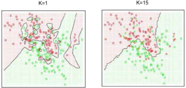
We already know that classification problem is predicting given input data into certain class. The simplest and most naive method is nearest neighbor. Given data training with class label, nearest neighbor classifier will assign given input data to the nearest data label. It can be done by using euclidean distance. Here is the illustration.

Continue reading “How k-NN (k-Nearest Neighbors) Works for Classification” →

How Gradient Descent Optimization Works for Minimizing Error

We already learn how we can use newton method to minimize error iteratively here. In this post, we will discuss about how we can use gradient descent method to minimize error interatively. When we later talk about neural network (deep neural network will be deep learning), we can say that understanding gradient descent is half of understanding neural network. And in fact, gradient descent is really easy to understand, likewise neural network. It’s true and not exaggerated 😀

Let’s talk about how gradient descent works first. This is also used in other machine learning methods, such as in logistic regression for binary classification here. Let’s assume we have function shown picture below to be minimized.

Continue reading “How Gradient Descent Optimization Works for Minimizing Error” →

Introduction to Classification and Confusion Matrix

In this machine learning and pattern recognition series, we already talk about regression problem that the output prediction is in continuous value. In machine learning, predicting output in discrete value given input is called classification. For two possible outputs, we usually call it as binary classification. For example, predicting that certain bank transaction is fraud or not, predicting that the cancer is benign or malignant, predicting that tomorrow will be raining or not, and so on. Whereas, for more than two possible outputs, we call it multi-class classification. For example, classification in hand gesture recognition whether the hand is moving right, left, bottom or up, classifying digit number 0 to 9, and so on.

Even thought classification is similar with regression, and the difference is only that classification output is discrete, whereas regression output is continuous, we can’t use exactly same method of regression for classification. The reason are : (1) it will perform bad when we classify given input to many classes, and (2) it lacks robustness to outliers. To use regression approach for classification, we need so-called activation function. Such method is called logistic regression, and we will talk later here. It is called logistic “regression” because we use similar way with what we did in regression here, but instead of taking output $y$ as prediction output, we feed the output $y$ into logistic function. The logistic function that is often used is sigmoid function. Furthermore, even its name uses “regression”, it is for classification problem, not regression problem. Continue reading “Introduction to Classification and Confusion Matrix” →

Bias-Variance Decomposition

During this post, we will try to decompose an error that actually an error consists of bias and variance. We will use MSE (mean square error) to define our error. Let $\theta$ is parameter we want to estimate, and $\hat{\theta}$ is our estimator result. Thus $MSE(\hat{\theta})=E[(\hat{\theta}-\theta)^2]$ and $bias(\hat{\theta})=E[\hat{\theta}-\theta]=E[\hat{\theta}]-\theta$ . Let’s decompose our MSE then.

$MSE = E[(\hat{\theta}-\theta)^2]=E[(\hat{\theta}-\mu-(\theta-\mu))^2]\\\\ MSE =E[(\hat{\theta}-\mu)^2-2(\hat{\theta}-\mu)(\theta-\mu)+(\theta-\mu)^2]\\\\ MSE =E[(\hat{\theta}-\mu)^2]-E[2(\hat{\theta}-\mu)(\theta-\mu)]+E[(\theta-\mu)^2]\\\\ MSE =E[(\hat{\theta}-\mu)^2]-2(\theta-\mu)E[(\hat{\theta}-\mu)]+(\theta-\mu)^2\,... \,(i)\\\\ MSE =E[(\hat{\theta}-\mu)^2]-2(\theta-\mu)(E[\hat{\theta}]-E[\mu])+(\theta-\mu)^2\\\\ MSE =E[(\hat{\theta}-\mu)^2]-2(\theta-\mu)(\mu-\mu)+(\theta-\mu)^2\\\\ MSE =E[(\hat{\theta}-\mu)^2]-2(\theta-\mu)(0)+(\theta-\mu)^2\\\\ MSE =E[(\hat{\theta}-\mu)^2]+(\theta-\mu)^2\\\\ MSE =E[(\hat{\theta}-E[\hat{\theta}])^2]+(\mu-\theta)^2\,... (ii)\,\\\\ MSE =E[(\hat{\theta}-E[\hat{\theta}])^2]+(E[\hat{\theta}]-\theta)^2\\\\ MSE = variance(\hat{\theta})+bias^2$ Continue reading “Bias-Variance Decomposition” →

Bayesian Linear / Polynomial Regression #Part2: Deriving Predictive Distribution

We already derive the posterior update formula $P(W|D)$ for Bayesian regression here, telling us that it is distribution of our parameter regression $\textbf{W}$ given data set $D$ . We are not directly interested in the value of $W$ , but, we are interested in the value of $Y$ itself given new value of new $x$ . This is exactly same with regression problem, given new value $x$ , we want to predict output value of $Y$ , which is in continuous value mode. And we already did linear regression problem using LSE (Least Square Error) here. During this post, we will do regression from Bayesian point of view. Using Bayesian in regression, we will have additional benefit. We will see later in the end of this post.

From #Part1 here, we already get $P(W|D)$ . To do regression in Bayesian point of view, we have to derive predictive distribution, so that we will have probability of $Y$ , $P(Y|\theta)$ . We can achieve that by doing marginalization. Here we go.