How Logistic Regression Works for Classification (with Maximum Likelihood Estimation Derivation)

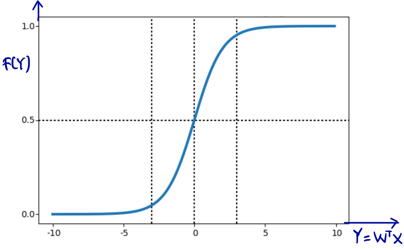
Logistic regression is an extension of regression method for classification. In the beginning of this machine learning series post, we already talked about regression using LSE here. To use regression approach for classification,we will feed the output regression into so-called activation function, usually using sigmoid acivation function. See piture below.

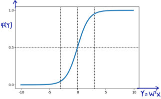
Sigmoid function will have output with s-shape like picture above whose output range is from zero to one. For classification, logistic regression is originally intended for binary classification. Regarding picture above, our output regression is fed sigmoid activation function. We will classify input to when the output is closed to 1 (formally when ) and classify to $class_2$ when the output is closed to 0 (formally when ) To do that, we can achieve by maximizing out likelihood using MLE (Maximum Likelihood Estiamtion).

We know that the output of our activation function is ranging from 0 to 1, and we also know that linear regression is originally intended for binary classification (two outcomes). Therefore, we can model our likelihood using product of Bernoulli distribution. If you are not really familiar with Bernoulli distribution, we already talked here and you can take a look of it. Given m-pair data training , here can be a vector such as . We can think that our each data , we have . And for , it is only or (binary class). Thus, our likelihood is product of Bernoulli distribution defined as follows.

To find that maximizes likelihood, we can take the first differential of our likelihood w.r.t , and make it equals to zero. As usual, to make it easier, we bring our likelihood to log form shown in the last line equation above.

Whoops! We are stuck here. We cannot find analytical function of that maximizes our likelihood, unlike what we did in LSE regression here that we could derive analytical form of that maximizes our loss function.

But, we have other methods to achieve this, maximizing our likelihood. We can use (1) gradient descent we already talk here, or (2) newton method for optimization we already talk here. Let’s break down for clearer understanding.

 

Using gradient descent to maximize likelihood in logistic regression

From our discussion here, we know that gradient descent formula is . In our logistic regression above, it will be.

We get the last line above since we already derive the first differential of our likelihood w.r.t . Given m-pair data training and n-order polynomial basis, we can write in matrix notation as follows.

where

.

And finally we can just this formula to train our logistic regression iteratively. In every iteration, we will try to maximize the likelihood until we get converged for our .

Using newton method to maximize likelihood in logistic regression

From our discussion about newton method for optimization here, we know that the formula is . It is for scalar form of . When  is a matrix, we can write , where is hessian matrix, that basically is second derivative of .

Using our newton method for formula above for optimization, we will try to derive the final formula for iteration update in our logistic regression case. Here we go.

To solve the differential term , we can use chain rule in differentiation. Let , and .

Plugging back our  result, we get.

We need to take transpose of in the last line of equation above since it’s square of vector. And we take the later of to be transposed because we know that this term should produce matrix.  Just like what we did in the gradient descent, we can write the matrix form of it and substitute , we get.

where is diagonal matrix x of . We prefer use because it is away more numerically stable when implementing into code in our computer. Then, we can just use this formula to train our logistic regression iteratively. Note that since this method needs inversing of our Hessian matrix, sometimes we find that our Hessian matrix is singular/not invertible.